Analzying GazePoint Pupil Data With GazeR

pupillometry

statistics

I demonstrate how to analyze pupil data from a GazePoint tracker with my eye-tracking R package gazeR.

Published

April 21, 2021

In this vignette I am going to show you how to read in a GazePoint data file along with some behavioral data and use gazeR to preprocess the data.

Special thanks to Matthew K Robinson (Twitter:@matthewkrobinson) for letting me use some data from an auditory oddball task he conducted on himself (we do what we have to do as researchers :D): see Tweet below.

To get started, we need to load in some important packages and read in the GP data files.

Load Packages

library(tidyverse)
library(remotes)
remotes::install_github("dmirman/gazer")
library(gazer)
library(data.table)
library(here)
remotes::install_github("tmalsburg/saccades/saccades", dependencies=TRUE)
library(saccades)

Read Data

pd <- fread('oddball_eye_13.tsv') # eye data 
bs<-fread('oddball_13.tsv') # behave data

head(pd)

     CNT     TIME    TIME_TICK    FPOGX     FPOGY    FPOGS   FPOGD FPOGID FPOGV
   <int>    <num>        <i64>    <num>     <num>    <num>   <num>  <int> <int>
1: 77433 1251.964 102150661899 -4.40518 -13.98604 1251.883 0.08093   1917     1
2: 77434 1251.980 102150821625 -4.39508 -13.95200 1251.883 0.09692   1917     1
3: 77435 1251.996 102150983307 -4.36427 -13.84678 1251.883 0.09692   1917     0
4: 77436 1252.013 102151149297 -4.40694 -13.99395 1251.883 0.09692   1917     0
5: 77437 1252.028 102151307171 -4.42096 -14.04383 1251.883 0.09692   1917     0
6: 77438 1252.045 102151469190 -4.40730 -14.00445 1251.883 0.09692   1917     0
     LPOGX   LPOGY LPOGV    RPOGX     RPOGY RPOGV    BPOGX     BPOGY BPOGV
     <num>   <num> <int>    <num>     <num> <int>    <num>     <num> <int>
1: 0.71795 0.50537     1 -9.38697 -28.00086     1 -4.33451 -13.74775     1
2: 0.71795 0.50537     1 -9.38697 -28.00086     1 -4.33451 -13.74775     1
3: 0.70711 0.51136     1 -9.14516 -27.18135     1 -4.21902 -13.33500     1
4: 0.70151 0.43055     1 -9.60071 -28.71280     1 -4.44960 -14.14113     1
5: 0.70270 0.42562     1 -9.60071 -28.71280     1 -4.44900 -14.14359     1
6: 0.69827 0.43625     1 -9.34484 -27.89350     1 -4.32329 -13.72862     1
      LPCX    LPCY      LPD     LPS   LPV    RPCX    RPCY      RPD   RPS   RPV
     <num>   <num>    <num>   <num> <int>   <num>   <num>    <num> <num> <int>
1: 0.34860 0.59214 25.23420 0.83829     1 0.64310 0.60511 28.49240     1     1
2: 0.34860 0.59216 25.27127 0.83829     1 0.64314 0.60509 28.33148     1     1
3: 0.34845 0.59234 25.09805 0.83829     1 0.64293 0.60517 28.69580     1     1
4: 0.34846 0.59237 25.15947 0.83829     1 0.64286 0.60519 28.47081     1     1
5: 0.34838 0.59240 25.32249 0.84484     1 0.64285 0.60518 28.46784     1     1
6: 0.34830 0.59240 25.07680 0.85139     1 0.64269 0.60527 28.50588     1     1
      LEYEX    LEYEY   LEYEZ LPUPILD LPUPILV   REYEX    REYEY   REYEZ RPUPILD
      <num>    <num>   <num>   <num>   <int>   <num>    <num>   <num>   <num>
1: -0.03362 -0.01726 0.56538 0.00455       1 0.03052 -0.01989 0.57411 0.00512
2: -0.03438 -0.01769 0.57821 0.00451       1 0.03056 -0.01997 0.57644 0.00513
3: -0.03438 -0.01769 0.57821 0.00449       1 0.03056 -0.01997 0.57644 0.00510
4: -0.03438 -0.01769 0.57821 0.00451       1 0.03056 -0.01997 0.57644 0.00509
5: -0.03501 -0.01795 0.58649 0.00448       1 0.03130 -0.02049 0.59132 0.00509
6: -0.03501 -0.01795 0.58649 0.00450       1 0.03130 -0.02049 0.59132 0.00508
   RPUPILV      CX      CY    CS  BKID BKDUR BKPMIN    LPMM LPMMV    RPMM RPMMV
     <int>   <num>   <num> <int> <int> <num>  <int>   <num> <int>   <num> <int>
1:       1 0.33333 0.33333     0     0     0     20 4.54567     1 5.11614     1
2:       1 0.33333 0.33333     0     0     0     20 4.51065     1 5.12683     1
3:       1 0.33333 0.33333     0     0     0     20 4.48607     1 5.10490     1
4:       1 0.33333 0.33333     0     0     0     20 4.50748     1 5.09460     1
5:       1 0.33333 0.33333     0     0     0     20 4.47957     1 5.08827     1
6:       1 0.33333 0.33333     0     0     0     20 4.50258     1 5.07552     1
    DIAL DIALV   GSR  GSRV    HR   HRV   HRP  TTL0  TTL1  TTLV            USER
   <num> <int> <int> <int> <int> <int> <int> <int> <int> <int>          <char>
1: 0.088     1     0     0     0     0   454    -1    -1     0               0
2: 0.088     1     0     0     0     0   484    -1    -1     0 STARTEXPERIMENT
3: 0.088     1     0     0     0     0   456    -1    -1     0 STARTEXPERIMENT
4: 0.088     1     0     0     0     0   451    -1    -1     0           START
5: 0.088     1     0     0     0     0   482    -1    -1     0           START
6: 0.088     1     0     0     0     0   454    -1    -1     0           START

head(bs)

   subject trial   tone    rt response
     <int> <int> <char> <int>   <char>
1:      13     1     lo  2113     None
2:      13     2     lo  2102     None
3:      13     3     lo  2107     None
4:      13     4     lo  2108     None
5:      13     5     lo  2107     None
6:      13     6     lo  2103     None

What we are going to do is run the GazePoint file through the merge_gazepoint function. The function below takes a list of files called file_list and merges all the files together, appends a subject column, creates a trial column using the USER column (GazePoint only allows messages through this channel), creates a time variable (in milliseconds). In the merge_gazepoint function the trail_msg argument requires users to denote a message used in the USER column that references the start of the trial–in our case the START message denotes the start of a new trial. This is a solution by Matt Robinson, but there are other ways one could extract the trial number. What I have done in the past is append a message with the trial iteration (e.g., START_1) in Python and use the separate function to get the trial number.

# A "monocular mean" averages both eyes together. If data is available in just
# one eye, use the available value as the mean, unless we need_both is TRUE.
#' @param x1 pupil left
#' @param x2 pupil right
#' @return vector with monocular mean values
compute_monocular_mean <- function(x1, x2) {
  xm <- rowMeans(cbind(x1, x2), na.rm = TRUE)
  # NaN => NA
  ifelse(is.nan(xm), NA, xm)
}


# function for processing GazePoint data
merge_gazepoint <- function (file_list, trial_msg = "START"){
  #file list is path to .xls files
  #vroom is faster
  library(data.table)
  
  file_ids=str_replace_all(basename(file_list),"([:alpha:]|[:punct:])","") # remove everything but numeric values
                   
  data <- map2(file_list, file_ids, ~fread(.x) %>% 
    mutate(id = .y))  %>% 
    bind_rows()

  
  d = data %>%
    dplyr::rowwise() %>%
    dplyr::mutate(pupil=compute_monocular_mean(RPMM, LPMM)) %>% # average both eyes
             dplyr::ungroup() %>%
           dplyr::mutate(pupil = ifelse(RPMMV == 0|LPMMV == 0, 0, pupil),  #missing data labeled as blinks
         new_trial = ifelse(USER == trial_msg & lag(USER) != trial_msg, 1, 0), # Label new trials
         trial = cumsum(new_trial), # Create a trial variable
         time = floor(TIME*1000)) %>%
    group_by(trial) %>%
    dplyr::mutate(time=time - min(time)) %>%
    ungroup() %>%
  dplyr::select(id, time,trial,pupil,BPOGX, BPOGY, USER) %>%
    dplyr::rename("message" = "USER", "subject"= "id", "x" = "BPOGX", "y" = "BPOGY") %>% 
    dplyr::filter(trial > 0)
  
  return(d)
}

Merge Files

setwd(here()) # setwd

gp_file<-list.files(here::here(), pattern = "eye_13.tsv") # get files 

setwd(here())
      
d=merge_gazepoint(gp_file, trial_msg = "START")

d$subject<-as.numeric(d$subject)

pdb <- full_join(bs, d)

pdb <- as_tibble(pdb)

pdb

# A tibble: 73,724 × 10
   subject trial tone     rt response  time pupil     x     y message
     <dbl> <dbl> <chr> <int> <chr>    <dbl> <dbl> <dbl> <dbl> <chr>  
 1      13     1 lo     2113 None         0  4.80 -4.45 -14.1 START  
 2      13     1 lo     2113 None        16  4.78 -4.45 -14.1 START  
 3      13     1 lo     2113 None        32  4.79 -4.32 -13.7 START  
 4      13     1 lo     2113 None        48  4.80 -4.58 -14.5 START  
 5      13     1 lo     2113 None        64  4.80 -4.58 -14.5 START  
 6      13     1 lo     2113 None        81  4.79 -4.63 -14.7 START  
 7      13     1 lo     2113 None        97  4.81 -4.42 -14.0 START  
 8      13     1 lo     2113 None       113  4.80 -4.42 -14.0 TONE   
 9      13     1 lo     2113 None       129  4.78 -4.23 -13.5 TONE   
10      13     1 lo     2113 None       145  4.77 -4.34 -13.8 TONE   
# ℹ 73,714 more rows

Blinks

Finding Blinks

The GazePoint data does not indicate where blinks occurred. What we are going to do is use the blink_detect function in gazer. This relies on the saccades package (https://github.com/tmalsburg/saccades) which uses a velocity based measure based on X,Y coordinates to find blinks. Once we find the blinks we can change the pupil size at that time point as NA and interpolate over it.

As a note, the GazePoint does not seem to sample consistently. In this case, it samples every 16 or 17 ms. This is a problem for some other blink detection measures (e.g., the noise based pupil function). One soultion would be to downsample the data at the onset so there is consistancy from sample to sample.

blinks_merge<- blink_detect(pdb)

 blinks <- blinks_merge %>%
        dplyr::group_by(grp = cumsum(!is.na(startend))) %>%
        dplyr::mutate(Label = replace(startend, first(startend) == 'start', 'start')) %>% #extends the start message forward until end message
        dplyr::ungroup() %>%
        # label blinks as 1
        dplyr::select(subject, trial, time, x, y, pupil, message, tone,  Label, -grp)
 
 
 blinks_data <- blinks  %>%
        dplyr::mutate(blink=ifelse(!is.na(Label), 1, 0), pupil=ifelse(blink==1 | pupil==0, NA, pupil))%>%
        dplyr::ungroup()%>%
        dplyr::select(subject, time, trial, pupil, x, y, trial, message, tone, blink, -Label)

Here is a look at the trials containing blinks:

blinks_data %>% 
  filter(blink==1) %>%
  head()%>%
  knitr::kable()

subject	time	trial	pupil	x	y	message	tone	blink
13	2167	10	NA	0.9364	1.95015	POSTTONE	lo	1
13	2183	10	NA	0.9364	1.95015	POSTTONE	lo	1
13	2199	10	NA	0.9364	1.95015	POSTTONE	lo	1
13	2216	10	NA	0.9364	1.95015	POSTTONE	lo	1
13	0	11	NA	0.9364	1.95015	START	hi	1
13	16	11	NA	0.9364	1.95015	START	hi	1

Extending Blinks

I am extending blinks 100 ms forward and backward in time.

Interpolate Blinks

Here let’s linearly interpolate the blinks and then smooth the data using a 5-point moving average.

# Smooth and Interpolate
smooth_interp <- smooth_interpolate_pupil(pup_extend, pupil="pupil", extendpupil="extendpupil", extendblinks=TRUE, step.first="smooth", maxgap=Inf, type="linear", hz=60, n=5)

Plot Interpolated Trial

interp_graph <- smooth_interp  %>%
  dplyr::filter(trial=="400")

bold <- element_text(face = "bold", color = "black", size = 14) #axis bold
#Graph interpolation
pup_g<- ggplot(interp_graph, aes(x= time, y= pupil)) + geom_point()+ geom_line(colour="black") +
  geom_line(aes(x=time, y=pup_interp), colour="darkgreen") + xlab("Time (ms)") + ylab("Pupil Size (mm)") + theme_bw() + theme(axis.title.y=element_text(size = 16, face="bold"), axis.title.x = element_text(size=16, face="bold"), axis.text.x=element_text(size = 12, face="bold"), axis.text.y=element_text(size=12, face="bold"))
print(pup_g)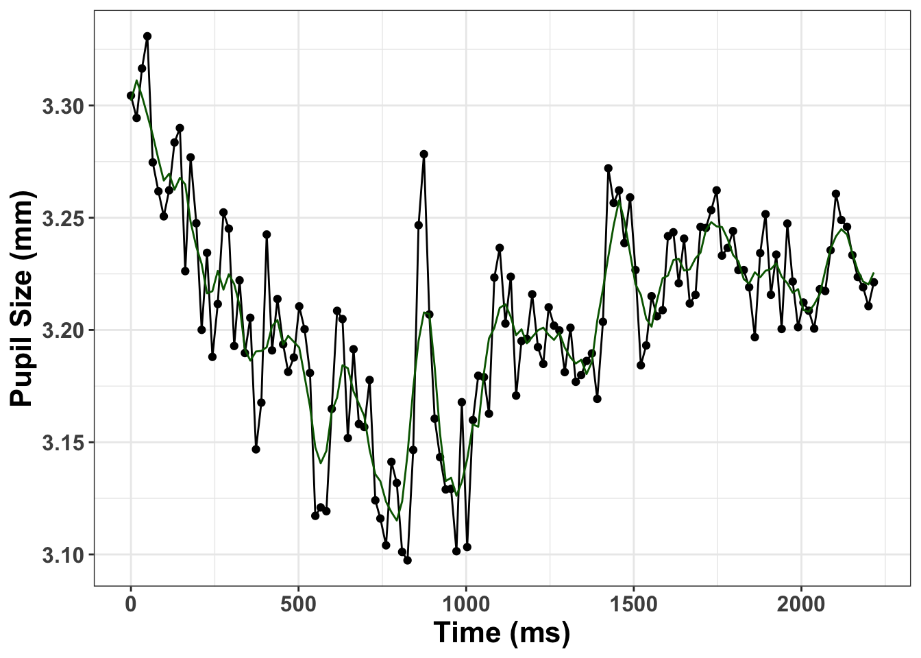

Baseline Correction

Here we will do a subtractive baseline correction taking 250 ms before the onset of the tone as baseline.

#use messages to baseline correct
baseline_pupil<-baseline_correction_pupil(smooth_interp, pupil_colname="pup_interp", baseline_window=c(0,250), baseline_method = "sub")

head(baseline_pupil)

# A tibble: 6 × 13
  subject trial baseline  time pupil     x     y message tone  blink extendpupil
    <dbl> <dbl>    <dbl> <dbl> <dbl> <dbl> <dbl> <chr>   <chr> <dbl>       <dbl>
1      13     1     4.80     0  4.80 -4.45 -14.1 START   lo        0        4.80
2      13     1     4.80    16  4.78 -4.45 -14.1 START   lo        0        4.78
3      13     1     4.80    32  4.79 -4.32 -13.7 START   lo        0        4.79
4      13     1     4.80    48  4.80 -4.58 -14.5 START   lo        0        4.80
5      13     1     4.80    64  4.80 -4.58 -14.5 START   lo        0        4.80
6      13     1     4.80    81  4.79 -4.63 -14.7 START   lo        0        4.79
# ℹ 2 more variables: pup_interp <dbl>, baselinecorrectedp <dbl>

Missing Data

Let’s see how much missing data there is and remove trials with greater than 20% missing data.

pup_missing<-count_missing_pupil(baseline_pupil, missingthresh = .5)
# remove outliers

I remove about 15 percent of trials.

Unlikely Pupil Sizes

Now let’s keep pupil diameter sizes between 2 mm and 9 mm

pup_outliers<-pup_missing %>%
  dplyr::filter (pup_interp  >= 2, pup_interp <= 9)

MAD

Get rid of artifacts we might have missed during some earlier steps.

  #MAD removal
max_removal<-pup_missing  %>%
  dplyr::group_by(subject, trial) %>%
  dplyr::mutate(speed=speed_pupil(pup_interp,time)) %>%
  dplyr::mutate(MAD=calc_mad(speed)) %>%
  dplyr::filter(speed < MAD)

Onset

Let’s only look fron the start of the trial until 1500 ms

baseline_pupil_onset<-max_removal %>%
  dplyr::group_by(subject, trial) %>%
  dplyr::filter(time <= 1500) %>%
  select(subject, trial, time,baselinecorrectedp, tone, time,message,baselinecorrectedp)

Downsample

Downsample the time-course to 50 ms.

#downsample
timebins1<- downsample_gaze(baseline_pupil_onset, bin.length=50, timevar = "time", aggvars = c("subject", "tone", "timebins"), type="pupil")

timebins1

# A tibble: 62 × 4
   subject tone  timebins aggbaseline
     <dbl> <chr>    <dbl>       <dbl>
 1      13 hi           0    0.00130 
 2      13 hi          50   -0.000752
 3      13 hi         100   -0.00206 
 4      13 hi         150    0.000331
 5      13 hi         200    0.00530 
 6      13 hi         250    0.00503 
 7      13 hi         300    0.00826 
 8      13 hi         350    0.00930 
 9      13 hi         400    0.0116  
10      13 hi         450    0.0125  
# ℹ 52 more rows

Visualize Time-course

cursive_plot <-ggplot(timebins1)+
  aes(timebins, aggbaseline, linetype=tone, color=tone) +
  stat_summary(fun = "mean", geom = "line", size = 1) +
  theme_bw() +
  labs(x ="Time (ms)",y ="Pupil Dilation (baseline - pupil))") +
  geom_hline(yintercept=0.0)

print(cursive_plot)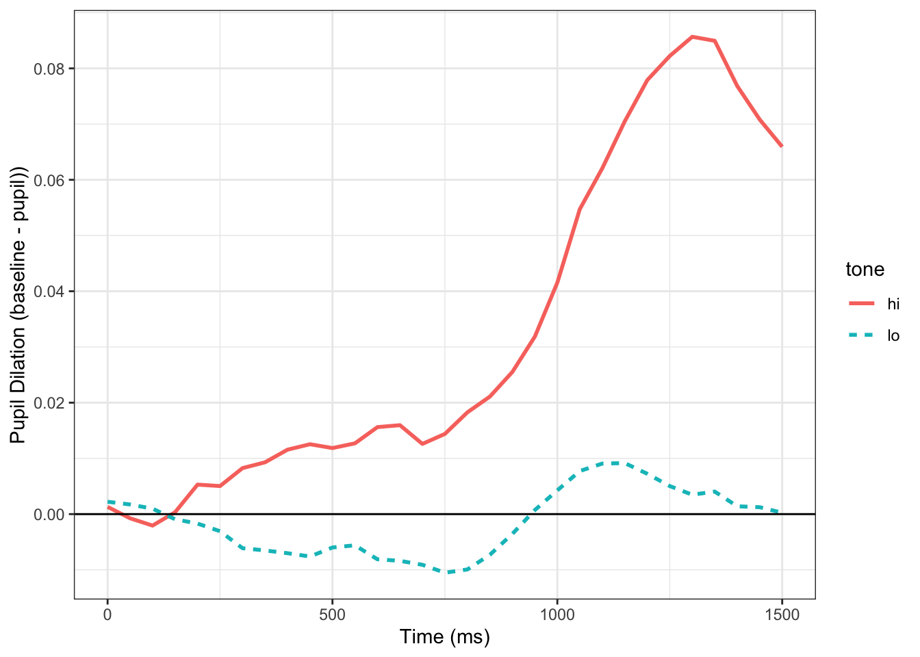

This looks very similar to the one in the Tweet albeit a bit smoother as a result of the extra preprocessing done.

Citation

BibTeX citation:

@online{2021,
  author = {},
  title = {Analzying {GazePoint} {Pupil} {Data} {With} {GazeR}},
  date = {2021-04-21},
  url = {https://www.drjasongeller.com/blog/posts/2021-04-21-gazePoint_gazer_2/},
  langid = {en}
}

For attribution, please cite this work as:

Analzying GazePoint Pupil Data With GazeR. (2021, April 21). https://www.drjasongeller.com/blog/posts/2021-04-21-gazePoint_gazer_2/